
What a Tennis Dampener Actually Dampens — A Student Research Case
Short answer: it makes the strings' “ping” die away 2.5 times faster, but it barely changes how the whole racket vibrates — the vibration that travels into your arm.
Before any numbers, put on headphones. These are two real recordings: same racket, same ball drop — one without a dampener, one with.
Both clips are scaled to the same peak loudness, so what you hear is how fast the sound dies, not how loud it is. With “only 549 Hz” on, a filter keeps just the strings' ping: without a dampener it drags a long tail; with one, it's gone almost at once.
1. Where the question came from
A dampener is a rubber button of about 2 grams, clipped between the two middle main strings. People say it “absorbs shock, protects your arm, prevents tennis elbow”. But two things vibrate when you hit a ball: the frame (the whole racket) and the string bed (the whole net of strings). The dampener only touches the strings — so which vibration does it actually reduce?
The experiment asks two questions:
2. How the experiment worked
Clamp the racket handle to a table, face up; drop a tennis ball onto the strings from a fixed height; record the “thwack–hmm” with a phone. Why sound? Because sound is a broadcast of vibration: however the strings and frame shake, the air shakes the same way. Take the sound apart and you can tell how long each vibration lasted.
| Data | Date | What | Recordings |
|---|---|---|---|
| A | 04-19 | no dampener vs dampener | 3 each, ~10 drops per recording |
| B1 | 08-30 | dampener on cross string 1, 4, 7, 10, 13 | 5 per position |
| B2 | 09-13 | added cross strings 16 and 19 | 5 per position |
In total: 41 recordings, about 28.6 minutes, 449 ball drops. Cross strings are counted from the throat (the handle end) upward: string 1 is nearest the handle, 19 nearest the tip, 10 in the middle.
3. The physics: three ideas are enough
① Vibration modes. When something is struck, it doesn't shake randomly — it vibrates in a few fixed “ways of singing” at once, each with its own pitch. Each way is a . A guitar string is the classic example: one pluck gives a fundamental plus overtones. A racket has two modes that matter most:
② Decay and σ. Every vibration fades, following exponential decay: amplitude ∝ e−σt. σ is the , in 1/second (s⁻¹). Bigger σ, faster fade. A friendlier number is : the time for the sound to drop by 60 (roughly, until you can't hear it). T60 = 6.908 ÷ σ.
Why decibels? On a plain scale the curve hugs zero almost immediately and the tail disappears. The decibel scale draws every “10× smaller” as the same step, so exponential decay becomes a straight line whose slope is σ.
③ A local damper. A dampener is like a finger resting lightly on the strings, turning vibration energy into heat. Press where the strings swing most (the middle) and it works best; press where they barely move (the ends) and it hardly works. In physics terms, the effect ∝ sin²(π·j/20), where j is the cross-string number — largest at string 10, near zero at both ends.
Turning the physics into predictions we can test:
| Prediction | Why | Result |
|---|---|---|
| The 549 Hz ping dies faster | rubber only touches strings | supported |
| The 118 Hz frame vibration is unchanged | 2 g is tiny next to a 300 g racket | supported |
| Overall ringing gets shorter | the ringing is mostly the ping | supported |
| The middle (string 10) works best | sin² | not settled |
4. Finding 1: the ping dies 2.5× faster
For each ball drop, a pulls out one mode, and we follow how its loudness falls over time (that curve is the ). Below is the median curve of 62 good drops:
5. Finding 2: the vibration that reaches your arm didn't change
Switch the chart above to 118 Hz: the blue and orange lines nearly overlap. The frame mode is the low-frequency vibration that travels down the handle into your arm, and the dampener hardly touches it. That matches scientists who measured the handle directly with accelerometers (Brody 1989; Li et al. 2004).
So: a dampener changes the sound and feel — the ping is gone, and hits sound duller and cleaner. Don't count on it to prevent tennis elbow.
6. Can we trust it?
We gave the result an exam: hide one recording, learn to tell “dampener or not” from the other five, then guess every drop in the hidden one. This is . The result:
Across all six: 58/62 right (93.5%). Using just one measure — “how much more the string-bed mode faded than the frame mode” — gets 61/62 (98.4%).
7. Finding 3: which string should it go on?
Tap a cross string on the racket to see what was measured there.
Three points:
① It works wherever you put it. At all seven positions the ping decays at 24–32 s⁻¹ — far from “no dampener” (11), close to “dampener” (32) (chart below).
Each dot is one recording (the median of its ~10 drops); the black line is the group median. Hover a dot for its value.
② On the same day, closer to the middle means less ringing. On 08-30, moving from string 1 to string 13 cut the leftover energy after the hit by 54%.
③ Past the middle, it may get weaker again. On 09-13, the ping decayed noticeably slower at string 19 (25.2) than at 16 (31.8) — the direction the sin² model predicts (string 19 is almost at the end of the strings). But careful — see the warning below.
8. Conclusions and next steps
| 1 | The dampener targets the string bed's ping (549 Hz), making it fade 2.5× faster. |
| 2 | It barely changes the frame vibration (118 Hz), so it changes sound and feel, not what reaches your arm. |
| 3 | It works on any string from 1 to 19; position only affects smaller things, and exactly how is still open. |
Next time, change these:
- Alternate “off / on” (off, on, off, on…) instead of recording all of one first.
- Record all positions on one day in random order; every day, also record “no dampener” and “string 10” as a reference.
- Write down the drop height, mic distance and how tight the clamp is.
- Tape a phone accelerometer to the handle to measure “what reaches the arm” directly.
Suppression of Impact Vibration by Tennis Racket Vibration Dampeners: An Experimental Study Based on Acoustic Modal Analysis, and the Effect of Mounting Position
Abstract
Purpose String vibration dampeners for tennis rackets are widely believed to "reduce vibration," but under amateur experimental conditions there is little quantitative evidence on what they actually act on (string-bed vibration or frame vibration), how large the effect is, and whether the mounting position matters. This study uses a phone microphone to record the sound radiated by a racket after a ball-drop impact, and answers these questions through mode-resolved decay analysis.
Methods The racket handle was clamped, and a tennis ball was dropped freely from a fixed height onto the center of the string bed; the impact sound was recorded with Audacity. Dataset A (2026-04-19): 3 tracks without a dampener (33 valid impacts) and 3 tracks with a dampener (29 valid impacts). Dataset B1 (2026-08-30): the dampener mounted at cross strings 1, 4, 7, 10, and 13, counted from the throat, with 5 tracks per position (264 valid impacts in total). Dataset B2 (2026-09-13): cross strings 16 and 19, with 5 tracks per position (102 valid impacts in total). A custom decoder recovered 44.1 kHz floating-point audio from the .aup3 projects; impacts were detected automatically, and ball-rebound and low-SNR events were removed. Four physical frequency bands were identified in the spectrum (the 118 Hz first frame bending mode, ~270 Hz, ~435 Hz, and the 549 Hz string-bed fundamental mode). For each impact we computed noise-aware narrowband envelope decay, broadband Schroeder decay, parameters of a two-exponential envelope model, and other metrics. The statistical analysis reports track-level (recording as the unit) permutation tests, event-level linear mixed-effects models (recording as a random effect), and hierarchical bootstrap confidence intervals; leave-one-track-out cross-validation was used to test whether the conclusions generalize. The position effect was fitted with linear, quadratic, and mode-shape sin² models and compared by cross-validation. Before comparing the two position recording sessions, their comparability was checked with setup metrics that "should not depend on dampener position."
Results (1) The effect of the dampener is highly mode-selective: without a dampener, the 549 Hz string-bed mode forms a slowly decaying tail that lasts beyond 0.4 s (tail level relative to the frame mode −14.9 ± 2.7 dB); with a dampener it falls to 60 dB below its peak within 0.2 s (tail relative level −23.9 ± 4.6 dB). The "extra decay of the string-bed mode relative to the frame mode" rises from −2.0 ± 4.2 dB to 16.9 ± 3.3 dB (difference 18.9 dB, 95% CI 16.3–21.4; Hedges' g = 4.9). The decay rate of the string-bed mode rises from 12.7 ± 6.2 s⁻¹ to 31.6 ± 4.2 s⁻¹ (ratio 2.5, 95% CI 2.1–3.0; T60 shortens from 0.62 s to 0.22 s, and the loss factor η increases from 0.007 to 0.019). (2) The 118 Hz frame mode is almost unaffected: decay over the 100 ms after the peak is 23.2 vs 22.9 dB, and the decay rate is 11.3 ± 4.6 vs 12.6 ± 3.4 s⁻¹ (ratio 1.11, CI 0.89–1.35). (3) Broadband metrics change accordingly: the residual energy fraction after 50 ms drops from 0.231 to 0.102 (ratio 0.44, CI 0.33–0.58), and the early decay time EDT drops from 0.390 s to 0.292 s; however, the slow component of the broadband two-exponential model (≈ 9 s⁻¹) is the same under both conditions and corresponds to the long tail of the frame mode rather than the string-bed mode. (4) Under leave-one-track-out cross-validation, the single feature "string-bed mode extra decay" alone distinguishes with vs without a dampener with 98.4% accuracy; the string-bed mode decay rate alone reaches 93.5%, and a four-feature logistic regression reaches 93.5%. (5) Mounting position: within the same recording session (B1), as the dampener moves from the throat (cross string 1) toward cross string 13, the residual energy fraction decreases overall (0.081 → 0.037, track-level Spearman ρ = −0.91, p < 0.001), the early spectral centroid rises from 311 Hz to 478 Hz, and the impact peak increases; the cross-validation error of the linear model is lower than that of the sin² mode-shape model centered at cross string 10. (6) The supplementary B2 data (cross strings 16 and 19) show that the 549 Hz string-bed mode is suppressed at all seven positions (track-median decay rates of 24–32 s⁻¹ at each position, far from the 11 s⁻¹ of the no-dampener control and close to the 32 s⁻¹ of the with-dampener control; this is a cross-session comparison and is only qualitative). However, the setup state clearly differed between the two recording sessions (frame mode decay rate about 11 vs 24–39 s⁻¹; ~270 Hz mode peak frequency 263 vs 291–296 Hz), so broadband ringing metrics cannot be compared directly across sessions. Within the same day, cross string 19 gives a lower string-bed mode decay rate than cross string 16 (25.2 vs 31.8 s⁻¹, track-level exact permutation p = 0.008), about 6 dB less extra decay relative to the frame (p = 0.03), and a longer EDT (p = 0.02); that is, the effect weakens past the center of the string bed, in the direction predicted by the sin² mode-shape model. In an exploratory pooled model that allows a session offset, the sin² model has the smallest cross-validation error for some endpoints, such as the residual energy fraction, EDT, and early spectral centroid; but it is equally "best" for the frame mode decay rate, which should not depend on position, showing that recording drift alone can produce this result. Because positions 16 and 19 were also recorded in sequence, and the frame frequency drifted by about 3 Hz between them, this evidence is only suggestive.
Conclusions The dampener removes the post-impact "ping" by applying strong damping to the string-bed fundamental mode, and has no measurable effect on the low-frequency frame mode, in agreement with the mechanical measurements of Brody (1989), Stroede et al. (1999), and Li et al. (2004). Mounted at any cross string from 1 to 19, the dampener suppresses the string-bed mode. Within the same recording session, the closer it is mounted to the center of the string bed (and thus to the impact point), the less residual ringing there is and the "crisper" the impact sound; past the center (cross string 19 vs cross string 16) there are signs that the effect weakens. Because the position experiments lack a same-day no-dampener baseline, position is confounded with recording order, and the setup state differed between the two recording sessions, the shape and mechanism of the position effect (mode-shape damping vs changed impact excitation) cannot yet be fully determined. This paper proposes an improved design that can bridge different recording sessions.
Keywords tennis racket; vibration dampener; damped vibration; modal analysis; decay time; mixed-effects model; cross-validation
1 Introduction
1.1 Background
When a tennis ball is hit, contact between the ball and the string bed lasts about 4–5 ms; afterward the string bed and the frame vibrate freely in their own natural modes, and the vibration is transmitted through the throat and handle to the arm. A string vibration dampener is a rubber button of about 2 g, clamped between the two central main strings, usually right next to the lowest cross string. Manufacturers and players commonly believe that it "reduces vibration and protects the arm," but existing mechanical studies give a more detailed picture: Brody (1989), using accelerometers, found that the dampener markedly shortens the duration of string vibration (about 500–600 Hz) but has no effect on frame vibration (100–200 Hz); Stroede et al. (1999) and Li et al. (2004) further confirmed that the dampener does not reduce the frame vibration transmitted to the handle and forearm. In other words, the dampener mainly changes sound and feel, not the low-frequency frame vibration that may cause tennis elbow.
For a high-school researcher, these results suggest a clear hypothesis that can be tested with low-cost equipment: if the dampener acts only on the string-bed mode, then in the spectrum of the impact sound the string-bed mode peak should disappear or decay faster when the dampener is fitted, while the frame mode peak should remain unchanged. A phone microphone and a free ball drop are enough to make this measurement.
1.2 Research Questions and Hypotheses
This study addresses two questions:
- Q1: How does the dampener affect the decay of each vibration mode after impact? How large is the effect?
- Q2: Does the mounting position of the dampener along the main strings (from the throat toward the center of the string bed) change its effect?
From these we formulate testable hypotheses:
| No. | Hypothesis | Theoretical basis (see Section 2) |
|---|---|---|
| H1 | The decay rate of the string-bed fundamental mode increases significantly, and its tail level more than 100 ms after impact decreases significantly | Viscoelastic energy dissipation in the rubber acts only on the strings it touches |
| H2 | The decay rate of the first frame bending mode is unchanged | The 2 g added mass and damping are negligible relative to the frame (~300 g) |
| H3 | Broadband "ringing" metrics (residual energy fraction, EDT, slow decay component) decrease accordingly | The slowly decaying tail is contributed by the string-bed mode |
| H4 | The string-bed mode frequency decreases slightly (mass loading; expected −1% to −4%) | Perturbation theory |
| H5 | The added damping is proportional to the square of the mode shape at the dampener location: the effect grows as the position moves from the throat toward the center, and saturates near the center | Local damper theory |
1.3 Analysis Strategy of This Study
Unlike the common approach of "looking at how fast the waveform decays," this paper emphasizes three points: (a) physical modes as endpoints: band-by-band analysis gives the conclusions a mechanical meaning and provides a built-in negative control; (b) gain-independent metrics first: absolute amplitudes are not comparable across recordings, whereas relative quantities within an event (such as the string-bed mode level relative to the frame mode level) are immune to confounders such as microphone distance and recording gain; (c) honest statistical units: each condition has only 3 recordings, and the 10 impacts within a track are not independent samples, so we report track-level tests, mixed-effects models, and cross-validation together.
2 Theoretical Background
2.1 Modes of the Racket–String-Bed System
The free vibration after impact can be written as a sum of damped harmonic modes:
$$x(t)=\sum_k A_k\,e^{-\sigma_k t}\cos(2\pi f_k t+\varphi_k),$$
where $f_k$ is the frequency of mode $k$ and $\sigma_k$ is the amplitude decay rate (s⁻¹). For a racket with a clamped handle, the main modes include the first frame bending mode (about 100–150 Hz), higher-order/hoop frame modes (about 300–500 Hz), and string-bed modes (about 500–700 Hz; Brody, Cross & Lindsey, 2002). The string-bed mode is formed by the whole string bed vibrating together like a membrane, and its fundamental frequency is approximately
$$f_1\approx\frac{1}{2L}\sqrt{\frac{T}{\mu_{\text{eff}}}},$$
where $L$ is the effective length of the main strings, $T$ is the tension, and $\mu_{\text{eff}}$ is the equivalent linear density taking the interwoven cross strings into account.
2.2 Decay Rate, T60, and Loss Factor
The amplitude of a single mode decays as $e^{-\sigma t}$, and its energy as $e^{-2\sigma t}$. In acoustics, the "time needed to drop by 60 dB" is commonly used:
$$T_{60}=\frac{\ln 10^{3}}{\sigma}=\frac{6.908}{\sigma},$$
The modal loss factor and quality factor are $\eta=\sigma/(\pi f)$ and $Q=1/\eta$. For a broadband signal containing several modes, the backward-integration method of Schroeder (1965) gives the energy decay curve (EDC)
$$\mathrm{EDC}(t)=\int_t^{\infty}x^2(\tau)\,d\tau,$$
T60 is obtained by extrapolating the slope of its −5…−25 dB segment, and the early decay time EDT from its 0…−10 dB segment (ISO 3382-1).
2.3 Local Damper: Added Damping Proportional to the Square of the Mode Shape
Attaching a small viscous damper (damping coefficient $c$) at position $x_d$ on a string produces, for mode $n$ (mode shape $\phi_n(x)=\sin(n\pi x/L)$, modal mass $M_n=\mu L/2$), an added decay rate of
$$\Delta\sigma_n=\frac{c\,\phi_n^2(x_d)}{2M_n}=\frac{c}{\mu L}\sin^2\!\left(\frac{n\pi x_d}{L}\right).$$
Therefore a dampener mounted at the end of the string (near a node) has almost no effect on the fundamental, while one mounted at the midpoint of the string (an antinode) has the largest effect. If the position is expressed by the cross-string index $j$, and the total number of cross strings plus one is $N$, then $x_d/L\approx j/N$. For a 16×19 string pattern $N\approx20$, and the predicted effect peaks near cross string 10 and falls off symmetrically (Figure 1b).
2.4 Frequency Shift Due to Mass Loading
By perturbation theory, an added mass $m$ lowers the modal frequency by
$$\frac{\Delta f_n}{f_n}\approx-\frac{m\,\phi_n^2(x_d)}{2M_n}.$$
Taking $m=2$ g, a string-bed modal mass of 4–8 g, and $\phi^2\approx0.05$–0.3 at the dampener, we get $\Delta f/f\approx-1\%$ to $-4\%$, i.e. a downward shift of 5–20 Hz near 549 Hz.
2.5 Testable Predictions
| Observable | Prediction (with vs without dampener) |
|---|---|
| Tail level of the 549 Hz string-bed mode | Significantly lower (disappears) |
| Post-peak decay of the 549 Hz mode | Significantly larger |
| Decay rate of the 118 Hz frame mode | Unchanged (negative control) |
| Broadband slow decay component | Lower amplitude fraction, higher decay rate |
| String-bed mode frequency | Decreases by 5–20 Hz |
| Position effect | Increases as $\sin^2(\pi j/N)$, saturating at the center |
3 Materials and Methods
3.1 Experimental Setup and Materials
The racket handle was clamped to a table (string face horizontal, facing up), and a tennis ball was released through a guide tube from a fixed height, landing on the center of the string bed (Figure 1a; see the photos in Figure 2). The dampener was a round button-type rubber dampener (diameter about 25 mm, mass about 2 g), mounted between the two central main strings. Sound was recorded with a phone microphone and saved as an Audacity project (44.1 kHz, mono, floating point). In dataset B, the first track for string 1 is named "5cm Trial 1", suggesting a ball-drop height of 5 cm for that batch; the other parameters (drop height, microphone distance) were not noted track by track in the original records, and this is discussed as a limitation in Section 5.4.
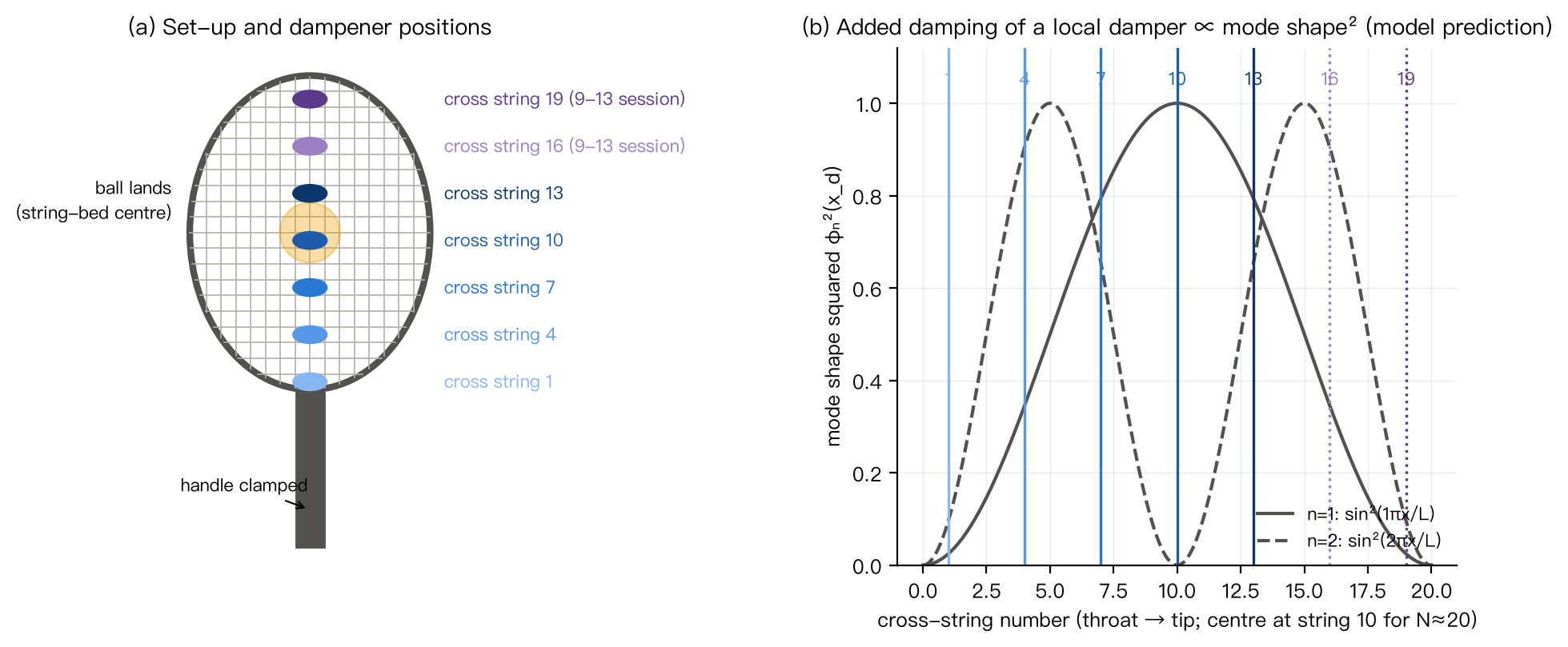
Figure 1. (a) Schematic of the setup and the dampener mounting positions (cross strings numbered from the throat toward the head); (b) local damper theory: the added damping is proportional to the square of the mode shape at that location; for N≈20 it is largest for the fundamental mode at cross string 10.
Figure 2 (racket structure and a photo of the dampener) used third-party images and is not reproduced on the web for copyright reasons.
3.2 Datasets
| Dataset | Recording date | Condition | Tracks | Impacts detected | Passed quality control |
|---|---|---|---|---|---|
| A (control) | 2026-04-19 | No dampener | 3 | 35 | 33 |
| With dampener | 3 | 30 | 29 | ||
| B1 (position) | 2026-08-30 | Cross string 1 | 5 | 53 | 51 |
| Cross string 4 | 5 | 57 | 53 | ||
| Cross string 7 | 5 | 57 | 52 | ||
| Cross string 10 | 5 | 55 | 54 | ||
| Cross string 13 | 5 | 59 | 54 | ||
| B2 (position) | 2026-09-13 | Cross string 16 | 5 | 52 | 52 |
| Cross string 19 | 5 | 51 | 50 |
Dataset B1 was recorded continuously in the order 1→4→7→10→13 (16:36–17:11), and had no same-day no-dampener baseline. Dataset B2 was recorded two weeks later; the file save times are 17:17 (cross string 16) and 17:21 (cross string 19). It was likewise recorded in sequence and has no no-dampener baseline. A 16×19 string pattern has 19 cross strings in total, and cross string 19 is the one closest to the head. B2 was provided in a zip archive dated 2026-09-22, which also contained the five B1 files (SHA-256 identical to the original files) and 16-bit WAV exports of the last track of each position file. The WAVs have a sample-by-sample correlation of 1.000 with the corresponding .aup3 tracks, but are clipped where |x| > 1, so they were not used.
3.3 Decoding and Integrity of the Raw Data
An .aup3 file is an SQLite database; samples are stored in blocks as little-endian float32, and the project structure is recorded as binary tokenised XML. A custom decoder (s01_extract_aup3.py) concatenates the samples according to waveblock.start, checks that the within-block extreme values match the database summaries, and records the SHA-256 of each source file. None of the 41 tracks is clipped (no flat plateaus; ≤ 2 samples at the maximum value). Sample magnitudes above 1 indicate that the student amplified the audio in Audacity; in floating-point format no information is lost.
3.4 Impact Event Detection and Quality Control
The impact onset is defined as follows: the |x| peak is ≥ 100 times the noise floor (the 10th percentile of the RMS in 50 ms windows), events are separated by ≥ 1.5 s, and the onset is found by tracing back from the peak to the point where the envelope stays below 5% of the peak for 2 ms continuously. For each event, 250–150 ms before onset is taken as the noise reference (the 150 ms just before onset is contaminated by pre-ringing from the zero-phase narrowband filters; see 3.5), and up to 0.6 s after onset is taken as the analysis window. Events are truncated or removed in the following cases (Figure 3):
- Ball rebound: the 20 ms smoothed envelope rises by ≥ 10 dB relative to its minimum over the previous 60 ms and is above −40 dB relative to the peak (detectable from 0.10 s at the earliest). Events with a rebound within 0.25 s are removed; otherwise the event is truncated 10 ms before the rebound. Events whose analysis window is shorter than 0.3 s after truncation are also removed;
- The peak occurs more than 30 ms after the onset (misdetected onset); the peak is below 50% of the track's median peak; SNR < 35 dB.
A total of 449 impacts were detected. 1 of them (the last impact in track 5 of cross string 19) lies only 0.30 s before the end of the recording, so its analysis window is incomplete and no metrics were computed. Of the remaining 448, 428 passed quality control and entered the analysis (all 102 B2 impacts with computed metrics passed).
3.5 Metric Definitions
Broadband metrics are computed on the signal after a 60–8000 Hz band-pass filter; modal metrics are computed band by band after a 40 Hz high-pass filter. Except for the peak amplitude, all metrics are independent of recording gain.
Broadband metrics - $t_{-20}$, $t_{-30}$: the time for the 5 ms RMS envelope to fall from the peak to −20/−30 dB; - Schroeder T60 (extrapolated from −5…−25 dB) and EDT (0…−10 dB); - Residual energy fraction: energy from 50 ms after impact to the end of the window / total energy; - Energy/peak²: the equivalent duration; - Two-exponential envelope model: $\hat A(t)=A_f e^{-\sigma_f t}+A_s e^{-\sigma_s t}+n$ ($n$ is the noise floor), fitted by least squares in the log domain from 10 ms to the end of the window; compared with a single-exponential model by AICc, where $\Delta\mathrm{AICc}>0$ means a slow component is needed.
Modal metrics (four fixed bands, 4th-order zero-phase Butterworth) - Bands: frame mode 100–135 Hz, ~270 Hz (240–300), ~435 Hz (410–460), string-bed mode 530–570 Hz; - 2.5 ms RMS envelope; the band noise floor is the RMS of the window 250–150 ms before onset. Zero-phase (filtfilt) narrowband filtering "drags" impact energy forward by about 100 ms (pre-ringing); if the 150 ms just before onset were also included in the noise window, the noise floor would be overestimated by more than 40 dB and the fit truncated too early (an early version of this study could barely fit the string-bed mode for this reason). Starting 10 ms after the peak, and using only samples more than 10 dB above the band's noise floor, $\ln A=\ln A_0-\sigma t$ is fitted (≥ 8 points) to obtain $\sigma$, T60, and $\eta$; - Decay (dB) over 100/250 ms after the peak; tail (150–300 ms) level; - Level relative to the frame mode: tail level of the string-bed band − tail level of the frame band; - Extra decay: (early 10–80 ms relative level) − (tail relative level), i.e. how many dB more the string-bed mode decays than the frame mode; this is a fully within-event, gain-independent quantity; - Modal frequency: the parabolically interpolated peak location of a zero-padded FFT over the 20–150 ms window.
3.6 Basis for Identifying the Modal Bands
For each of the six recordings in dataset A, we computed the per-event median PSD (Welch, 4096 points, s05b_track_psd.py) of the ringing window (30–300 ms) and the tail window (100–400 ms). The per-frequency-bin median level difference between the two groups over 60–2000 Hz is only 0.3–0.6 dB, showing that the recording gain was consistent; the differences are concentrated in a few peaks: 549 Hz (tail about 16 dB higher without a dampener), 250–290 Hz (tail median about 7 dB higher), and 430–450 Hz (2–4 dB higher), while the 118 Hz peak almost coincides between the groups (Figure 5). On this basis the four bands above were fixed. 118 Hz agrees with the first frame bending mode of a clamped racket reported by Brody et al., and 549 Hz lies in the range of the string-bed fundamental.
3.7 Statistical Analysis
Unit of analysis Each condition has 3 recordings with about 10 impacts each. Impacts within a track share the same setup state and cannot be treated as independent. Therefore, for each endpoint we report: 1. Track level: Welch t-test and exact permutation test (20 assignments; smallest attainable p = 0.10) on the per-track medians (n = 3 vs 3); 2. Event-level linear mixed-effects model: $y\sim\text{condition}+(1\,|\,\text{track})$ (REML; positive-valued metrics are log-transformed and the estimate is reported as a ratio), giving the estimate, 95% CI, and p; 3. Hierarchical bootstrap: first resample recordings, then resample events within recordings (4000 times), giving 95% percentile intervals for the difference of means and the ratio of means; 4. Event-level Hedges' g as the effect size.
Position effect: trend statistics are computed only within one recording session (B1): Kruskal–Wallis test and Spearman trend on the track-level medians (5 per position); event-level Spearman with cluster bootstrap CIs; and the mixed-effects model $y\sim\text{position}+(1\,|\,\text{track})$. B2 has only two positions, so cross strings 16 and 19 are compared with an exact permutation test on 5 vs 5 track medians (all 252 groupings; smallest attainable p = 0.008), Hedges' g, and the mixed-effects model. Before combining the two recording sessions, we first compare setup metrics that in theory are not affected by dampener position (frame mode decay rate and frequency, ~270 Hz mode peak frequency, noise floor). The significance level is 0.05 and no multiple-comparison correction is applied, but primary endpoints (H1–H3) are distinguished from exploratory endpoints according to the prespecified hypotheses.
3.8 Modeling and Cross-Validation
- Classification cross-validation (dataset A): leave-one-track-out (LOTO) logistic regression with four gain-independent features (string-bed mode 100 ms decay, extra decay, residual energy fraction, EDT; standardized); the LOTO accuracy of single-feature threshold rules is also evaluated.
- Position models (dataset B1): five models are fitted to the track-level medians: constant, linear, quadratic, $a+b\sin^2(\pi j/20)$, and $a+b\sin^2(\pi j/N)$ ($N$ free, 14–30), compared by the RMSE of leave-one-track-out and leave-one-position-out cross-validation and by AICc.
- Seven-position pooled model (B1 + B2, exploratory): each model receives a B2 session offset term (constant + session, linear + session, $\sin^2(\pi j/20)$ + session), again compared by AICc and leave-one-track-out and leave-one-position-out CV. Because B2 has only positions 16 and 19, the session offset can only be estimated by relying on the assumed curve shape, so the results are for reference only.
3.9 Software and Reproducibility
Python 3.12 with NumPy, SciPy, pandas, statsmodels, scikit-learn and Matplotlib. The whole analysis can be rebuilt from the raw recordings with a single command, and two rebuilds give byte-identical results.
4 Results
4.1 Data Quality
A total of 449 impacts were detected in the 41 tracks; metrics were computed for 448 (1 lies at the end of a recording), and 428 passed quality control (Figure 3). The SNR of valid impacts is 36–70 dB (median 55 dB; 53–65 dB for B2). In dataset B1, 8 ball rebounds earlier than 0.25 s were detected and removed, and another 7 events were removed because their analysis window was shorter than 0.3 s after truncation; in A and B1, 5 events in total (3 in A, 2 in B1) were removed because their peaks were too small; in B2, 4 ball rebounds were detected (0.33–1.37 s, all later than 0.25 s, truncated only), and none of the events with computed metrics was removed. The noise floors of the two control conditions are similar, but the impact peak in the with-dampener recordings is about 1.9 times that of the no-dampener recordings (6.29 ± 1.84 vs 3.31 ± 0.58 a.u.). Because the frame mode level differs by only 3–5 dB between the groups (much less than the 5.6 dB difference in peak), this difference more likely reflects a change in the impact transient itself or a difference in the relative microphone position, rather than gain; absolute amplitude is therefore used only as a secondary metric.
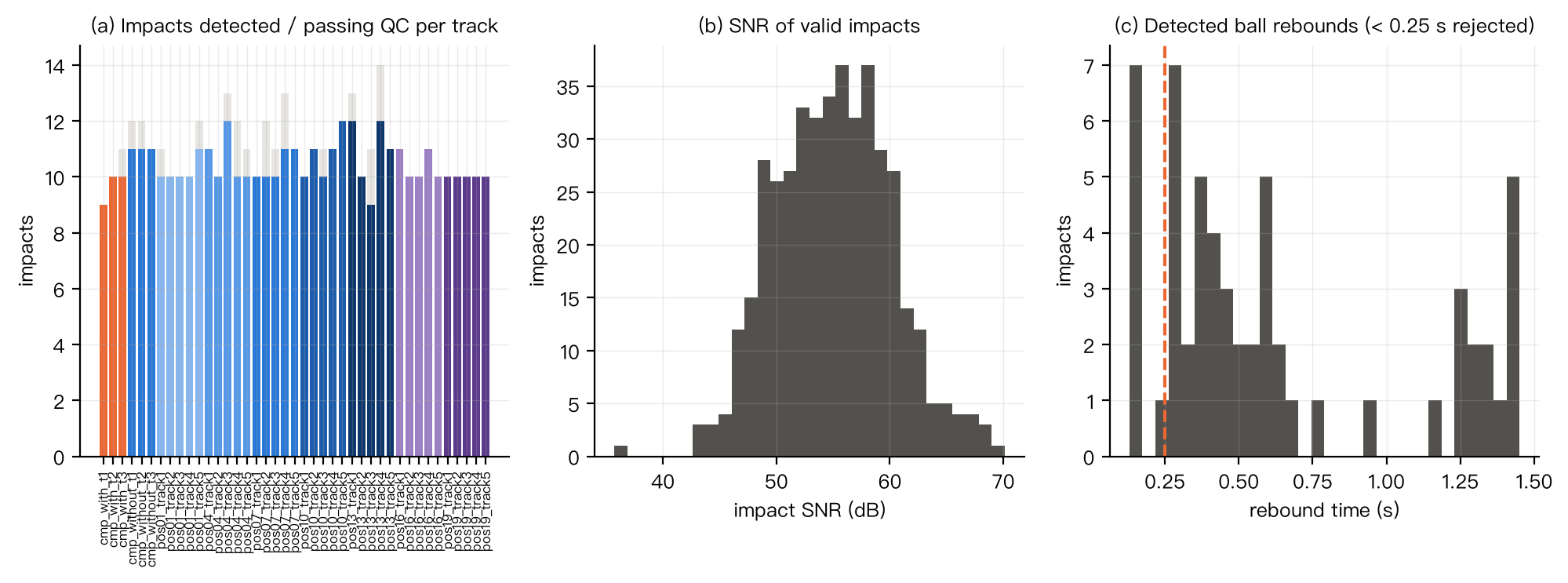
Figure 3. Data quality control: (a) number of impacts detected and passing quality control per track; (b) SNR of valid impacts; (c) distribution of detected ball rebound times.
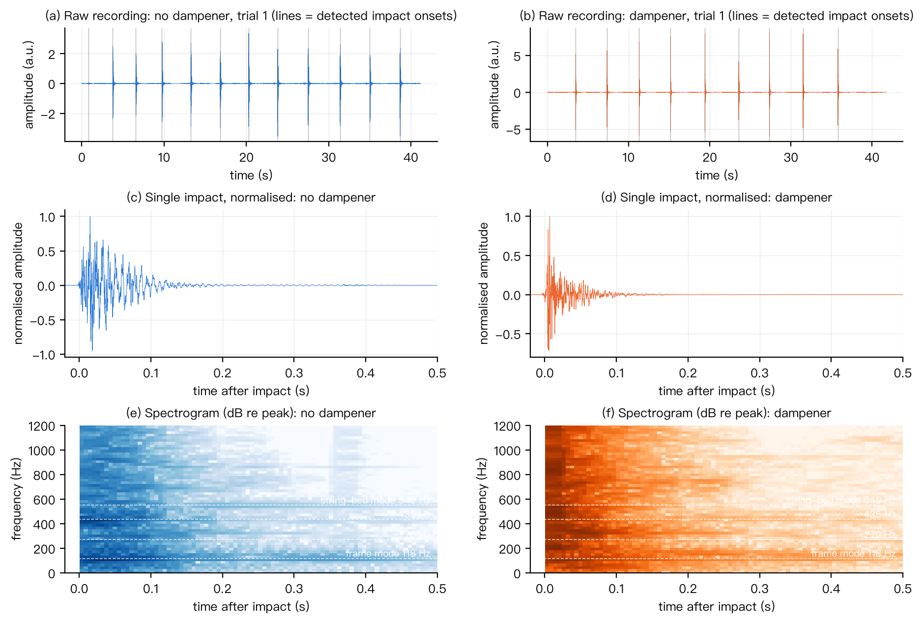
Figure 4. (a,b) Raw control recordings (vertical lines mark the detected impact onsets); (c,d) normalized waveforms of single impacts; (e,f) spectrograms. Without a dampener, persistent horizontal bright lines are visible at 118, 435, and 549 Hz; with a dampener, the 549 Hz line disappears.
4.2 Identifying the Dampener-Sensitive Modes
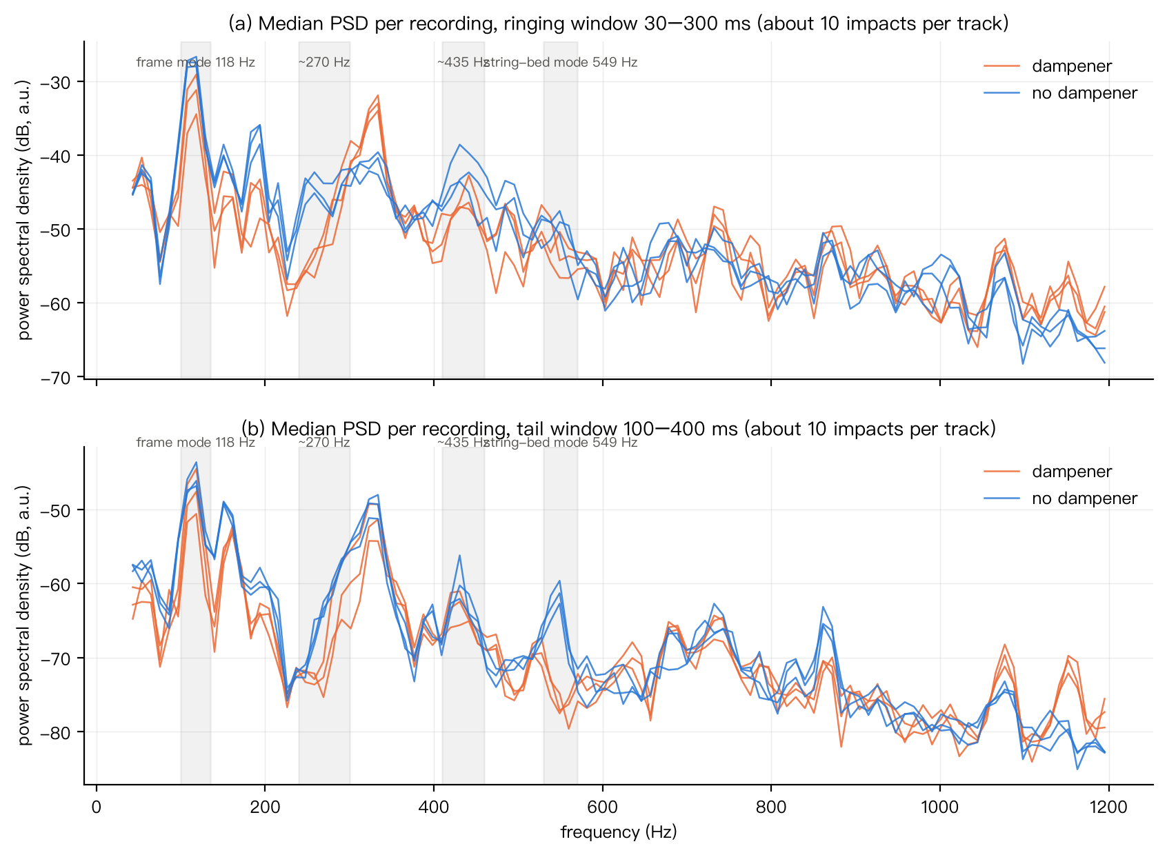
Figure 5. Median power spectrum of each control recording: (a) ringing window 30–300 ms; (b) tail window 100–400 ms. Gray bands mark the four analysis bands.
Figure 5 shows that the six recordings have consistent levels at the 118 Hz frame mode (tail −44 to −51 dB), whereas 549 Hz shows a sharp contrast: at the 549 Hz bin, the tail spectra of the three no-dampener recordings show a peak of −60 to −63 dB, while the three with-dampener recordings show only a background of −75 to −78 dB (the three-track medians differ by about 16 dB). In the 250–290 Hz region the no-dampener tail median is about 7 dB higher (with one with-dampener recording as an exception), and at 430–450 Hz it is 2–4 dB higher; in the ringing window, around 330 Hz the with-dampener level is about 7 dB higher, which may correspond to a local mode of the dampener and strings. This pattern is highly consistent across the three repeated recordings.
4.3 Decay of the String-Bed Mode (H1) and Invariance of the Frame Mode (H2)
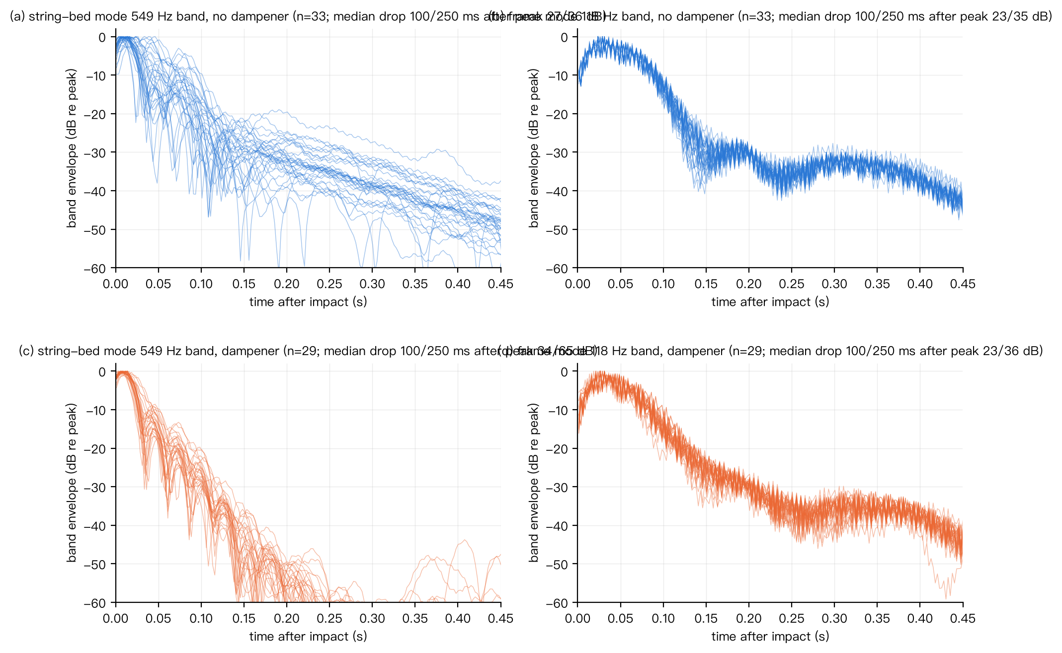
Figure 6. Per-event envelopes (dB re band peak) of the 549 Hz string-bed band (left) and the 118 Hz frame band (right). Top row: no dampener; bottom row: with dampener.
Figure 6 is the core evidence of this study. Without a dampener (a), the 549 Hz band first drops quickly by about 25 dB after impact, then decays slowly with a slope of about −6 dB / 0.1 s, and is still above −50 dB at 0.45 s. An exponential fit over the whole segment from 10 ms after the peak to noise floor +10 dB (0.33 s on average) gives a decay rate σ = 12.7 ± 6.2 s⁻¹ (track medians 9.2, 12.5, 11.2 s⁻¹), T60 = 0.62 ± 0.18 s, and loss factor η = 0.007. With a dampener (c), the same band falls below −60 dB within 0.2 s; the fitted segment (0.19 s on average, spanning 54 dB) gives σ = 31.6 ± 4.2 s⁻¹ (track medians 32.2, 33.0, 32.5 s⁻¹), T60 = 0.22 ± 0.03 s, and η = 0.019, a 2.5-fold increase in decay rate (bootstrap 95% CI 2.1–3.0). In contrast, the envelopes of the 118 Hz frame band (b, d) almost coincide under the two conditions: the decay over 100/250 ms after the peak is 23.2/35.2 dB (without) and 22.9/35.7 dB (with), and the whole-segment fitted σ is 11.3 ± 4.6 and 12.6 ± 3.4 s⁻¹.
Table 1 summarizes the primary endpoints (full table in Appendix A).
Table 1. Primary endpoints for the control group (mean ± SD; mixed-effects model estimates; hierarchical bootstrap 95% CI)
| Endpoint | No dampener (n=33) | Dampener (n=29) | Difference or ratio [bootstrap 95% CI] | Hedges' g | Mixed-model p | Track permutation p |
|---|---|---|---|---|---|---|
| String-bed extra decay (dB) | -2.0 ± 4.2 | 16.9 ± 3.3 | +18.9 [16.3, 21.4] | 4.88 | 3×10⁻⁵⁵ | 0.10 |
| Tail string-bed level re frame (dB) | -14.9 ± 2.7 | -23.9 ± 4.6 | -9.0 [-11.7, -6.1] | -2.39 | 1×10⁻¹⁰ | 0.10 |
| String-bed drop 100 ms after peak (dB) | 27.2 ± 6.8 | 34.5 ± 5.5 | +7.3 [3.3, 11.8] | 1.16 | 3×10⁻⁴ | 0.10 |
| String-bed drop 250 ms after peak (dB) | 35.9 ± 4.4 | 63.9 ± 4.0 | +28.0 | — | — | — |
| String-bed decay rate σ (s⁻¹) | 12.7 ± 6.2 | 31.6 ± 4.2 | ×2.49 [2.10, 2.99] | 3.52 | 1×10⁻³⁴ | 0.10 |
| String-bed T60 (s) | 0.62 ± 0.18 | 0.22 ± 0.03 | ×0.36 [0.31, 0.41] | -3.00 | 1×10⁻³⁴ | 0.10 |
| String-bed loss factor η | 0.0074 ± 0.0036 | 0.0187 ± 0.0024 | +0.0113 | — | — | — |
| Frame decay rate σ (s⁻¹) | 11.3 ± 4.6 | 12.6 ± 3.4 | ×1.11 [0.89, 1.35] | 0.31 | 0.04 | 0.10 |
| Frame-mode drop 100 ms after peak (dB) | 23.2 ± 4.0 | 22.9 ± 2.6 | -0.3 | — | — | — |
| Frame-mode drop 250 ms after peak (dB) | 35.2 ± 1.4 | 35.7 ± 1.7 | +0.6 | — | — | — |
| Residual energy fraction (>50 ms) | 0.231 ± 0.042 | 0.102 ± 0.051 | ×0.44 [0.33, 0.58] | -2.76 | 2×10⁻¹⁵ | 0.10 |
| EDT (s) | 0.390 ± 0.024 | 0.292 ± 0.062 | ×0.75 [0.67, 0.83] | -2.10 | 5×10⁻¹⁰ | 0.10 |
| t₋₂₀ (s) | 0.111 ± 0.010 | 0.087 ± 0.017 | ×0.79 [0.69, 0.89] | -1.73 | 2×10⁻⁴ | 0.10 |
| t₋₃₀ (s) | 0.157 ± 0.009 | 0.127 ± 0.019 | ×0.81 [0.73, 0.90] | -2.04 | 2×10⁻⁵ | 0.10 |
| Schroeder T60 (s) | 0.288 ± 0.016 | 0.274 ± 0.019 | ×0.95 [0.89, 1.01] | -0.80 | 0.15 | 0.60 |
| Two-exp. slow component σ_s (s⁻¹) | 8.6 ± 2.4 | 10.1 ± 7.6 | ×1.17 [0.83, 1.60] | 0.27 | 0.41 | 1.00 |
| Two-exp. slow amplitude share | 0.062 ± 0.033 | 0.077 ± 0.158 | +0.014 [-0.029, 0.103] | 0.13 | 0.12 | 0.10 |
| ΔAICc (single − two-exp.) | 54 ± 33 | 65 ± 42 | +10.8 [-10.8, 30.2] | 0.29 | 0.26 | 0.20 |
| String-bed frequency (Hz) | 547.2 ± 13.1 | 540.0 ± 15.9 | -7.3 [-18.8, 4.1] | -0.50 | 0.21 | 0.50 |
| Frame-mode frequency (Hz) | 113.2 ± 0.5 | 114.8 ± 0.6 | +1.6 [1.1, 2.1] | 2.92 | 1×10⁻⁸ | 0.10 |
| Impact peak (a.u.) | 3.31 ± 0.58 | 6.29 ± 1.84 | ×1.90 [1.62, 2.20] | 2.22 | 4×10⁻¹⁹ | 0.10 |
| Energy / peak² (s) | 0.0060 ± 0.0014 | 0.0028 ± 0.0016 | ×0.47 [0.35, 0.62] | -2.07 | 1×10⁻¹⁶ | 0.10 |
Note: in a 3 vs 3 design, the smallest attainable p for the track-level permutation test is 0.10; reaching this value means that the medians of all three with-dampener recordings lie outside those of all three no-dampener recordings.
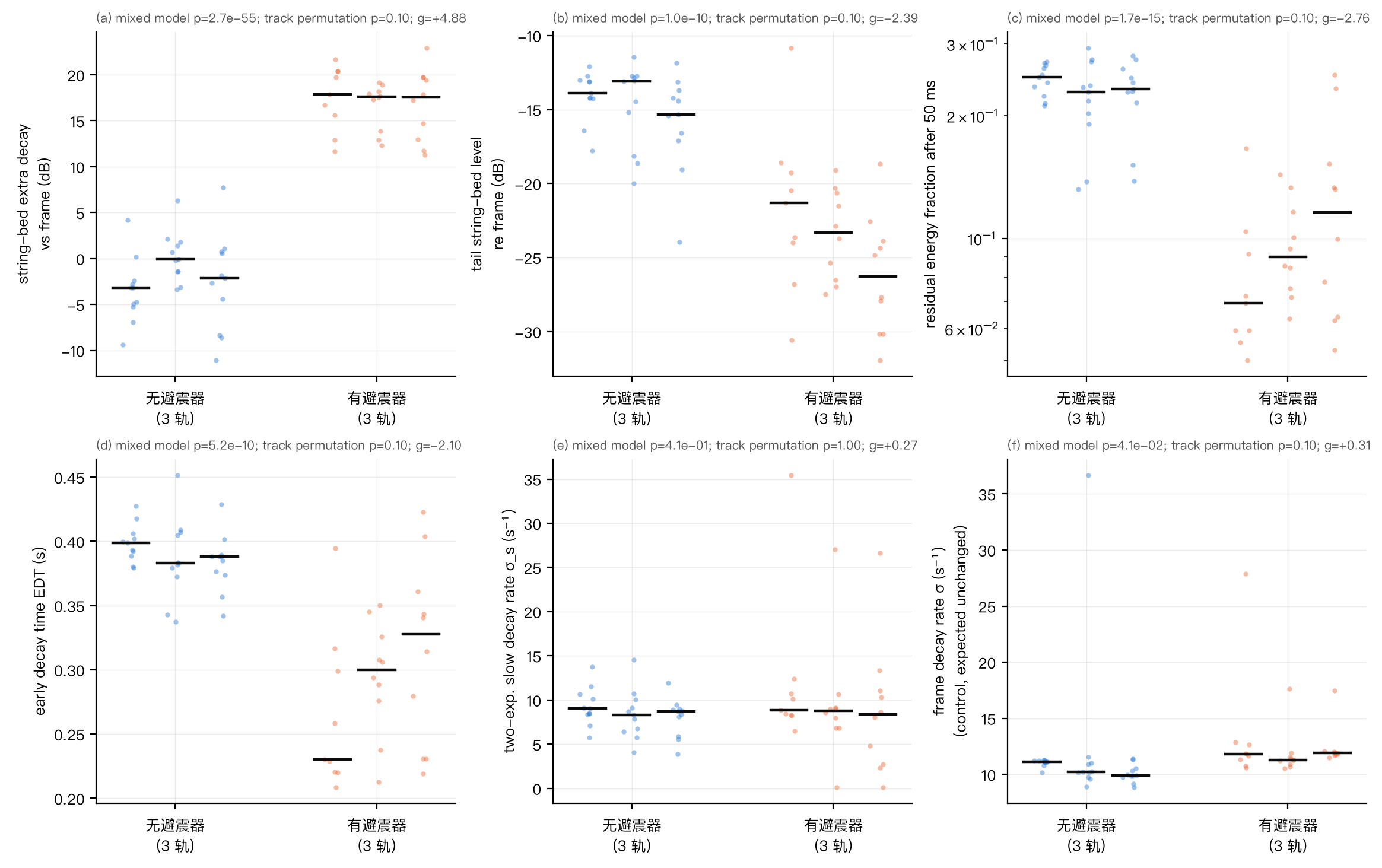
Figure 7. Event-level distributions and per-track medians of the primary endpoint metrics. (a) String-bed mode extra decay; (b) tail level of the string-bed mode relative to the frame; (c) residual energy fraction (log axis); (d) EDT; (e) decay rate of the two-exponential slow component (same for both conditions); (f) frame mode decay rate (negative control).
H1 is strongly supported: three independently defined string-bed mode metrics agree, and the medians of all three with-dampener recordings lie outside the range of the three no-dampener recordings (Figure 7a–b), with within-track spread much smaller than the between-group difference. H2 is also supported: the fixed-window decay of the frame mode is the same, and although the CI of the ratio of whole-segment fitted decay rates (0.89–1.35) leans slightly toward faster decay with the dampener (mixed-effects model p = 0.04), this is negligible compared with the 2.5-fold change in the string-bed mode.
4.4 Broadband Decay and the Two-Exponential Model (H3)
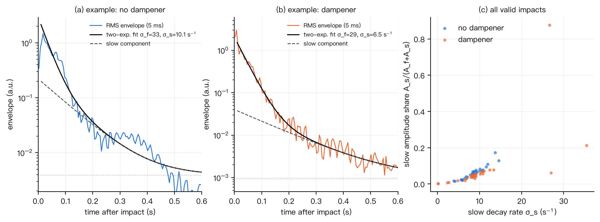
Figure 8. Broadband two-exponential envelope model. (a) No-dampener example: a fast component σ_f ≈ 33 s⁻¹ superimposed on a slow component σ_s ≈ 10 s⁻¹; (b) with-dampener example: a slow component of σ_s ≈ 7–10 s⁻¹ is also present; (c) distribution of (σ_s, slow-component fraction) for all valid impacts; the two conditions overlap.
Under both conditions the broadband envelope requires a two-exponential description (events with ΔAICc > 0: 94% and 86%), and the decay rate of the slow component is the same (8.6 vs 10.1 s⁻¹, ratio 1.17, CI 0.83–1.60). Comparing with Figure 6b/d shows that this slow component is the long tail of the 118 Hz frame mode near −35 dB, which the dampener does not change. Although the 549 Hz string-bed mode also lasts to 0.4 s without a dampener, its tail level is about 15 dB below that of the frame mode, and the broadband model cannot separate these two components with similar decay rates (≈ 9 and ≈ 13 s⁻¹). In other words, the effect of the dampener is not obvious in the shape of the broadband envelope and can only be seen band by band. Even so, the energy of the string-bed mode within 50–300 ms is enough to change broadband energy metrics: the residual energy fraction halves, EDT shortens by 25%, and t₋₂₀ and t₋₃₀ shorten by about 20%. Notably, Schroeder T60 (the −5…−25 dB segment) is insensitive to the dampener (ratio 0.95, CI includes 1), because this segment is dominated by the rapidly decaying impact transient. This shows that for impact-type signals, EDT and the residual energy fraction are better "ringing" metrics than T60.
4.5 Frequency Shift (H4)
With a dampener, the string-bed mode frequency is 7.3 Hz lower (−1.3%), in the direction predicted by mass loading, but the bootstrap CI (−18.8 to +4.1 Hz) includes zero; moreover, with a dampener there is no longer a clear modal peak in this band, so the frequency estimate mainly reflects the broadband background. H4 can therefore only be regarded as "not contradicted." On the other hand, the frame mode frequency differs by 1.6 Hz between the groups (1.4%, mixed-effects model p ≈ 1×10⁻⁸). A 2 g dampener cannot raise the frame frequency; this difference more likely comes from a difference in clamping state between the two groups of recordings, and it serves as an internal indicator that "the setup was not exactly the same for the two groups of recordings" (see 5.4).
4.6 Cross-Validation
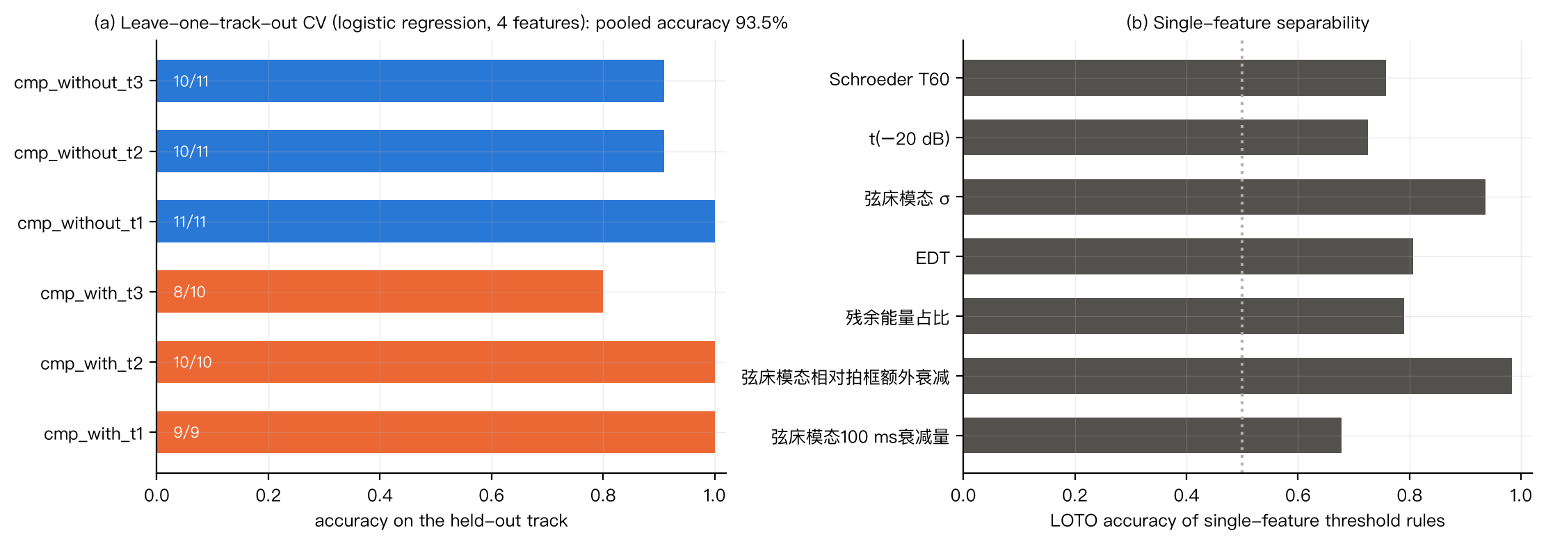
Figure 9. (a) Leave-one-track-out cross-validation: per-impact classification accuracy on the held-out recording of a logistic regression trained on the other 5 recordings; (b) leave-one-track-out accuracy of single-feature threshold rules.
The pooled leave-one-track-out accuracy of the four-feature logistic regression is 93.5% (58/62); the accuracies on the six held-out recordings are 9/9, 10/10, 8/10, 11/11, 10/11, and 10/11. The single feature "string-bed mode extra decay" alone reaches 98.4% (61/62), and the string-bed mode decay rate σ reaches 93.5%, both far higher than the broadband metrics (EDT 80.6%, residual energy fraction 79.0%, T60 75.8%). This shows that: (i) the dampener effect generalizes to unseen recordings rather than being a peculiarity of one recording; (ii) mode-resolved metrics have much better discriminating power than broadband metrics.
4.7 Mounting Position Effect (B1: 2026-08-30, Cross Strings 1–13)
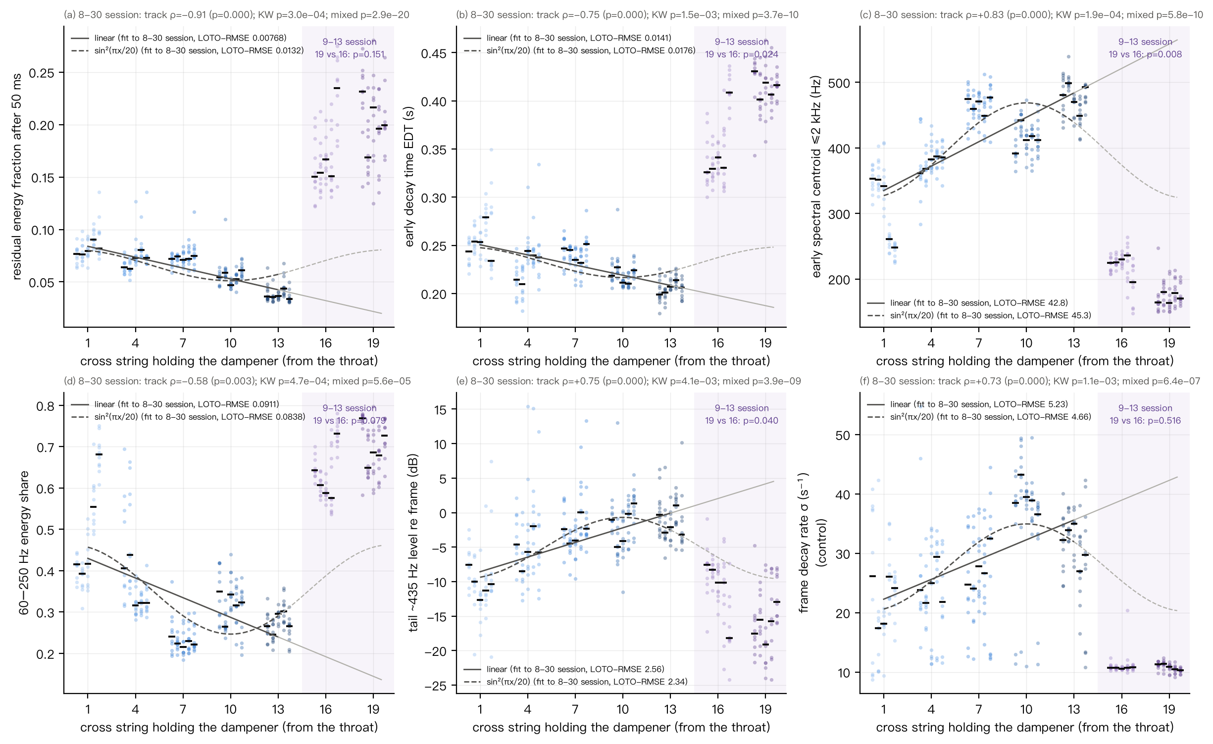
Figure 10. Relationship between mounting position (cross-string index counted from the throat) and each endpoint. Dots = single impacts, black lines = per-track medians (5 tracks per position), solid line = linear fit, dashed line = sin² mode-shape model centered at cross string 10; both are fitted only to B1 (cross strings 1–13), and the light gray lines are their extrapolations beyond cross string 13. Titles give the B1 track-level Spearman ρ, Kruskal–Wallis p, and mixed-effects model slope p. The purple shading marks cross strings 16 and 19 from the other recording session (B2), with the track-level exact permutation p between them in the upper right. The difference in absolute level between B2 and B1 mainly reflects a different setup state (see 4.9), and the points should not be read as one continuous curve along the horizontal axis.
Table 2. Position means (mean of the 5 track medians per position) and trend statistics for each endpoint in position group B1 (full table in Appendix C)
| Endpoint | String 1 | String 4 | String 7 | String 10 | String 13 | Track-level ρ (p) | Event-level ρ [95% CI] | Mixed-model p |
|---|---|---|---|---|---|---|---|---|
| Residual energy fraction | 0.081 | 0.071 | 0.073 | 0.055 | 0.037 | -0.91 (<0.001) | -0.81 [-0.89, -0.64] | 3×10⁻²⁰ |
| EDT (s) | 0.253 | 0.229 | 0.242 | 0.218 | 0.205 | -0.75 (<0.001) | -0.67 [-0.81, -0.44] | 4×10⁻¹⁰ |
| Early spectral centroid (Hz) | 311 | 377 | 466 | 415 | 478 | +0.83 (<0.001) | +0.74 [+0.49, +0.86] | 6×10⁻¹⁰ |
| 700–2000 Hz energy share | 0.14 | 0.17 | 0.23 | 0.22 | 0.35 | +0.83 (<0.001) | +0.79 [+0.58, +0.89] | 2×10⁻¹⁰ |
| 60–250 Hz energy share | 0.49 | 0.36 | 0.23 | 0.32 | 0.27 | -0.58 (0.003) | -0.57 [-0.76, -0.22] | 6×10⁻⁵ |
| Tail ~435 Hz level re frame (dB) | -10.4 | -5.3 | -2.7 | -1.8 | -1.5 | +0.75 (<0.001) | +0.56 [+0.34, +0.70] | 4×10⁻⁹ |
| Tail string-bed level re frame (dB) | -21.2 | -13.6 | -11.9 | -13.5 | -11.7 | +0.57 (0.003) | +0.44 [+0.18, +0.63] | 2×10⁻⁵ |
| Impact peak (a.u.) | 1.10 | 1.19 | 1.39 | 1.40 | 1.69 | +0.83 (<0.001) | +0.64 [+0.44, +0.77] | 6×10⁻¹² |
| Frame decay rate (s⁻¹) | 22.4 | 24.3 | 27.1 | 39.3 | 31.6 | +0.73 (<0.001) | +0.45 [+0.28, +0.57] | 6×10⁻⁷ |
| ~435 Hz mode decay rate (s⁻¹) | 29.4 | 25.0 | 21.4 | 16.9 | 16.4 | -0.78 (<0.001) | -0.43 [-0.54, -0.29] | 8×10⁻⁹ |
| Frame-mode frequency (Hz) | 114.4 | 112.8 | 115.2 | 116.4 | 116.7 | +0.78 (<0.001) | +0.73 [+0.55, +0.79] | 0.001 |
| Broadband envelope decay rate (s⁻¹) | 25.1 | 25.6 | 26.2 | 26.3 | 24.6 | -0.02 (0.926) | -0.05 [-0.31, +0.26] | 0.99 |
| t₋₃₀ (s) | 0.113 | 0.119 | 0.132 | 0.126 | 0.105 | -0.12 (0.559) | -0.16 [-0.42, +0.18] | 0.27 |
The position effect shows a clear and selective pattern:
- Less ringing: the residual energy fraction drops by 54% from cross string 1 to cross string 13 (0.081 → 0.037); the five track medians do not overlap at all among cross strings 7, 10, and 13, while adjacent positions among cross strings 1–7 overlap (Figure 10a); EDT drops by 19%.
- A "crisper" impact: the early (10–80 ms) spectral centroid rises by 54%, the 700–2000 Hz energy fraction increases 2.5-fold, the 60–250 Hz fraction halves, and the impact peak rises by 53% (Figure 10c, d and Figure 11). These are changes in the excitation spectrum, not in the decay rate.
- Broadband decay rate unchanged, but the frame mode drifts: the broadband envelope decay rate and t₋₃₀ show no trend; the frame mode decay rate, however, rises from 22 to 39 s⁻¹ (Figure 10f), in step with a +2.3 Hz drift in its frequency. Tighter clamping would raise both the frame frequency and its damping, so this looks more like a change in the clamp state during recording than an effect of dampener position (a 2 g dampener cannot change the frame mode). The decay rate of the ~435 Hz mode falls from 29 to 16 s⁻¹ with position, consistent with the rise in its tail relative level.
- The tail relative level of the 435 Hz mode rises with position and tends to saturate (−10.4 → −1.5 dB, Figure 10e).
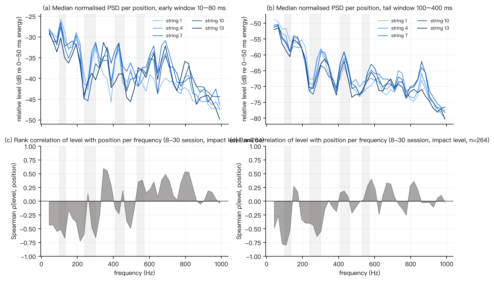
Figure 11. (a,b) Median normalized PSD at each position (referenced to the 0–50 ms impact energy); (c,d) Spearman rank correlation between per-bin level and position. Components at 80–300 Hz decrease as the position moves toward the center, and components at 550–600 Hz and above 700 Hz increase.
4.8 Comparison of Position Models (H5, Within Session B1)
Table 3. Model comparison on track-level medians (LOTO = leave-one-track-out CV-RMSE, LOPO = leave-one-position-out CV-RMSE; bold marks the minimum in each column)
| Endpoint | Model | Parameters | R² | AICc | LOTO | LOPO |
|---|---|---|---|---|---|---|
| Residual energy fraction | Constant | — | 0.00 | -203.7 | 0.0170 | 0.0201 |
| Linear | 0.08738 − 0.00346·j | 0.81 | -242.7 | 0.0077 | 0.0102 | |
| Quadratic | 0.07873 + 0.000449·j − 0.000279·j² | 0.88 | -250.8 | 0.0064 | 0.0108 | |
| sin²(πj/20) | 0.0807 − 0.0296·sin² | 0.42 | -214.7 | 0.0132 | 0.0166 | |
| sin²(πj/N), N free | 0.08255 − 0.0415·sin², N = 30 (boundary) | 0.80 | -239.5 | 0.0078 | 0.0214 | |
| EDT | Constant | — | 0.00 | -194.0 | 0.0206 | 0.0234 |
| Linear | 0.2541 − 0.00352·j | 0.57 | -212.6 | 0.0141 | 0.0150 | |
| Quadratic | 0.2504 − 0.00186·j − 0.000118·j² | 0.58 | -210.5 | 0.0146 | 0.0235 | |
| sin²(πj/20) | 0.2483 − 0.0318·sin² | 0.33 | -201.5 | 0.0176 | 0.0212 | |
| sin²(πj/N), N free | 0.2488 − 0.0415·sin², N = 30 (boundary) | 0.55 | -208.7 | 0.0144 | 0.0270 | |
| ~435 Hz tail level | Constant | — | 0.00 | 69.2 | 3.98 | 4.55 |
| Linear | -9.282 + 0.708·j | 0.62 | 47.4 | 2.56 | 3.42 | |
| Quadratic | -12.07 + 1.97·j − 0.0901·j² | 0.75 | 39.9 | 2.17 | 2.19 | |
| sin²(πj/20) | -9.591 + 8.9·sin² | 0.69 | 42.6 | 2.34 | 2.79 | |
| sin²(πj/N), N free | -9.5 + 8.76·sin², N = 20.8 | 0.69 | 44.8 | 2.40 | 3.54 | |
| 60–250 Hz share | Constant | — | 0.00 | -109.6 | 0.111 | 0.127 |
| Linear | 0.4458 − 0.0159·j | 0.40 | -119.8 | 0.091 | 0.118 | |
| Quadratic | 0.5445 − 0.0605·j + 0.00319·j² | 0.60 | -127.3 | 0.079 | 0.122 | |
| sin²(πj/20) | 0.4623 − 0.216·sin² | 0.51 | -125.1 | 0.084 | 0.109 | |
| sin²(πj/N), N free | 0.4664 − 0.225·sin², N = 18.8 | 0.52 | -123.1 | 0.085 | 0.146 |
For the ringing metrics (residual energy fraction, EDT), the cross-validation error of the sin² model centered at cross string 10 is clearly larger than that of the linear model; when N is left free, the fit converges to the search boundary N = 30, meaning the data over 1–13 are monotonic, with no saturation, which does not match the "saturation at the center, symmetric fall-off" predicted by H5. Only the 435 Hz mode relative level and the 60–250 Hz fraction show saturation, where the sin² model and the quadratic model perform similarly. Note that 1–13 covers only the rising part of the sin² curve and the region near its top; the difference between the linear and sin² shapes over this range lies mainly at cross strings 10 and 13. What can really distinguish the two are positions beyond cross string 10, which is exactly why B2 added cross strings 16 and 19 (4.9).
4.9 The Second Position Session (B2: 2026-09-13, Cross Strings 16 and 19)
(1) The two recording sessions cannot be merged directly. Table 4 lists setup metrics that in theory are unrelated to the dampener mounting position. The frame mode decay rate in B2 is about 11 s⁻¹, less than half of that in B1 (24–39 s⁻¹), and the same as the 10–12 s⁻¹ of the control group (2026-04-19). The median ~270 Hz mode peak frequency in B2 is 262–264 Hz (one recording at cross string 19 is at 295 Hz), about 30 Hz lower than in B1 (291–296 Hz) and the control group (296–303 Hz); the noise floor of B2 is also lower than that of B1. A 2 g dampener can neither halve the frame damping nor shift a mode down by 30 Hz, so these differences can only come from changes in setup state (clamping method and force, string tension or condition, microphone position, etc.). Therefore, the large differences between B2 and B1 in broadband metrics such as the residual energy fraction, EDT, and the 60–250 Hz fraction (purple region in Figure 10) are mainly a result of the frame mode ringing longer in B2, not an effect of positions 16 and 19 themselves.
Table 4. Setup consistency metrics for each recording group (median of per-track medians; range across tracks in square brackets)
| Session | Group | Tracks | Frame σ (s⁻¹) [track range] | Frame-mode frequency (Hz) | ~270 Hz peak frequency (Hz) [track range] | ~435 Hz peak frequency (Hz) | String-bed σ (s⁻¹) | Noise floor (×10⁻⁴) |
|---|---|---|---|---|---|---|---|---|
| 2026-04-19 | No dampener | 3 | 10.2 [9.9–11.1] | 113.2 | 298 [296–300] | 433 | 11.2 | 6.4 |
| 2026-04-19 | Dampener | 3 | 11.8 [11.3–11.9] | 114.6 | 303 [302–303] | 441 | 32.5 | 6.6 |
| 2026-08-30 | String 1 | 5 | 24.1 [17.4–26.2] | 114.1 | 291 [290–292] | 431 | 30.8 | 11.0 |
| 2026-08-30 | String 4 | 5 | 23.8 [21.7–29.4] | 114.0 | 293 [292–293] | 430 | 24.6 | 11.0 |
| 2026-08-30 | String 7 | 5 | 26.7 [24.0–32.5] | 114.8 | 296 [295–297] | 429 | 25.6 | 10.9 |
| 2026-08-30 | String 10 | 5 | 38.9 [36.5–43.2] | 116.5 | 295 [293–296] | 428 | 24.4 | 6.8 |
| 2026-08-30 | String 13 | 5 | 32.2 [27.0–35.0] | 116.7 | 295 [293–295] | 428 | 27.9 | 7.2 |
| 2026-09-13 | String 16 | 5 | 10.7 [10.6–10.8] | 115.4 | 264 [263–273] | 425 | 31.8 | 5.8 |
| 2026-09-13 | String 19 | 5 | 10.9 [10.3–11.4] | 112.4 | 262 [262–295] | 431 | 25.2 | 5.6 |
(2) The string-bed mode is suppressed at all seven positions. The decay rate of the string-bed mode itself (looking only at the 530–570 Hz band, without referencing the frame) has track medians of 24–32 s⁻¹ at each position from cross string 1 to 19, all far from the 11 s⁻¹ of the no-dampener control and close to the 32 s⁻¹ of the with-dampener control (Figure 12c; this is a cross-session comparison and should be read only qualitatively, since there are still differences between positions; for example, on the same day cross string 19 is significantly lower than cross string 16, see below). The decay over 250 ms after the peak is 54–62 dB, also close to the with-dampener value (67 dB) and far greater than the no-dampener value (35 dB). In other words, whichever cross string it is mounted at, the dampener removes the 549 Hz "ping"; position changes only secondary effects.
(3) Within the same day, cross string 19 is less effective than cross string 16. Table 5 compares the two positions within B2 (5 recordings each). At cross string 19 the string-bed mode decay rate is lower (25.2 vs 31.8 s⁻¹, g = −5.0, exact permutation p = 0.008, the smallest value attainable in a 5 vs 5 design), the decay over 100 ms after the peak is 4 dB less, and the extra decay relative to the frame is about 6 dB less (17.8 → 11.6 dB); in broadband terms, EDT is longer (0.33 → 0.42 s), the early spectral centroid is lower (226 → 170 Hz), and the tail relative level at ~435 Hz is lower. According to local damper theory, the squared mode shape sin²(πj/20) at cross strings 16 and 19 is 0.35 and 0.02 respectively; cross string 19 is almost at the end of the string, and the predicted added damping is clearly smaller. The observed direction agrees with this and is opposite to a linear extrapolation of "the closer to the head, the better."
Table 5. Cross string 19 vs cross string 16 within session B2 (full table in Appendix E)
| Endpoint | String 16 (median of 5 track medians) | String 19 | 19 − 16 (difference of means) | Hedges g | Track-level exact permutation p (252 splits) | Mixed-model p |
|---|---|---|---|---|---|---|
| String-bed decay rate σ (s⁻¹) | 31.8 | 25.2 | -7.6 | -5.04 | 0.008 | 1×10⁻⁷ |
| String-bed extra decay vs frame (dB) | 17.8 | 11.6 | -5.7 | -2.05 | 0.032 | 2×10⁻⁵ |
| String-bed drop 100 ms after peak (dB) | 32.1 | 29.0 | -4.1 | -1.56 | 0.016 | 0.04 |
| Residual energy fraction | 0.154 | 0.200 | +0.031 | +0.92 | 0.151 | 0.04 |
| EDT (s) | 0.330 | 0.416 | +0.068 | +2.35 | 0.024 | 5×10⁻⁵ |
| Early spectral centroid (Hz) | 226 | 170 | -51 | -3.70 | 0.008 | 1×10⁻⁹ |
| 60–250 Hz energy share | 0.61 | 0.69 | +0.07 | +1.19 | 0.079 | 0.03 |
| Tail ~435 Hz level re frame (dB) | -10.1 | -15.8 | -5.3 | -1.41 | 0.040 | 0.01 |
| Impact peak (a.u.) | 1.40 | 1.67 | +0.28 | +2.03 | 0.016 | 5×10⁻⁴ |
| Frame decay rate (s⁻¹) | 10.7 | 10.9 | +0.1 | +0.36 | 0.516 | 0.58 |
| Frame-mode frequency (Hz) | 115.4 | 112.4 | -2.8 | -3.17 | 0.008 | 1×10⁻⁶ |
However, this comparison is also confounded by order: the two files were recorded 4 minutes apart in the order 16 → 19, and during that time the frame mode frequency dropped by about 3 Hz (track medians 115.4 → 112.4 Hz, p = 0.008), showing that the setup drifted even within one day. The impact peak rises with recording order in both B1 (1 → 13) and B2 (16 → 19) (B2: 1.40 → 1.67, p = 0.016), which most likely reflects mainly drift during recording rather than dampener position.
(4) Seven-position models with a session offset (exploratory). Table 6 combines B1 and B2 and adds a "B2 session offset" to each model. For the residual energy fraction, EDT, early spectral centroid, ~435 Hz tail relative level, and 60–250 Hz fraction, the sin²(πj/20) + session model has the smallest AICc and the smallest leave-one-track-out and leave-one-position-out CV errors of the three models, the opposite of the conclusion from B1 alone, where the linear model was preferred. For the impact peak, the 700–2000 Hz fraction, and the tail level of the string-bed mode relative to the frame, the linear + session model is better; for the string-bed mode extra decay there is no consistent winner (AICc and leave-one-track-out favor linear + session, leave-one-position-out favors constant + session). An important counterexample: for the frame mode decay rate, which in theory is unrelated to dampener position, the pooled sin² + session model is also "best" (AICc 100.6 vs 106.5 for linear + session), because in B1 the frame damping drifted up and then down during recording, which happens to give a "high in the middle" shape. In other words, recording drift alone can make the sin² model win. Combined with the fact that the session offset can only be estimated from the assumed shape (B2 has only two positions), this result only shows that "the data do not contradict the mode-shape model and do not support an effect that increases monotonically with position"; it cannot serve as evidence that H5 holds.
Table 6. Model comparison over seven positions with a session offset (track-level medians; bold marks the minimum in each column; the last column is the comparison using B1 only; full table in Appendix F)
| Endpoint | Model | Session offset | Shape coeff. | AICc | LOTO | LOPO | 8-30 session only: linear / sin² LOTO |
|---|---|---|---|---|---|---|---|
| Residual energy fraction | Constant + session | +0.1236 | — | -263.8 | 0.0235 | 0.0278 | 0.0077 / 0.0132 |
| Linear + session | +0.153 | -0.002799 | -270.3 | 0.0213 | 0.0285 | ||
| sin²(πj/20) + session | +0.1095 | -0.03467 | -271.4 | 0.0207 | 0.0234 | ||
| EDT | Constant + session | +0.1514 | — | -247.0 | 0.0299 | 0.0430 | 0.0141 / 0.0176 |
| Linear + session | +0.1752 | -0.002275 | -248.0 | 0.0292 | 0.0469 | ||
| sin²(πj/20) + session | +0.1329 | -0.04529 | -255.3 | 0.0261 | 0.0377 | ||
| Early spectral centroid | Constant + session | -212.7 | — | 288.1 | 60.3 | 73.3 | 42.8 / 45.3 |
| Linear + session | -328.4 | +11.02 | 266.6 | 44.8 | 66.8 | ||
| sin²(πj/20) + session | -153.4 | +146 | 256.0 | 38.7 | 52.3 | ||
| ~435 Hz tail level | Constant + session | -9.202 | — | 99.4 | 4.13 | 5.06 | 2.56 / 2.34 |
| Linear + session | -15.39 | +0.5897 | 88.8 | 3.57 | 5.25 | ||
| sin²(πj/20) + session | -5.348 | +9.478 | 71.4 | 2.78 | 3.03 | ||
| 60–250 Hz share | Constant + session | +0.331 | — | -159.5 | 0.101 | 0.117 | 0.091 / 0.084 |
| Linear + session | +0.4775 | -0.01395 | -168.8 | 0.090 | 0.122 | ||
| sin²(πj/20) + session | +0.243 | -0.2165 | -180.9 | 0.076 | 0.092 | ||
| String-bed extra decay | Constant + session | +4.282 | — | 95.0 | 3.87 | 4.74 | 3.73 / 3.65 |
| Linear + session | +8.136 | -0.367 | 92.2 | 3.69 | 4.86 | ||
| sin²(πj/20) + session | +3.233 | -2.579 | 95.6 | 3.93 | 5.80 |
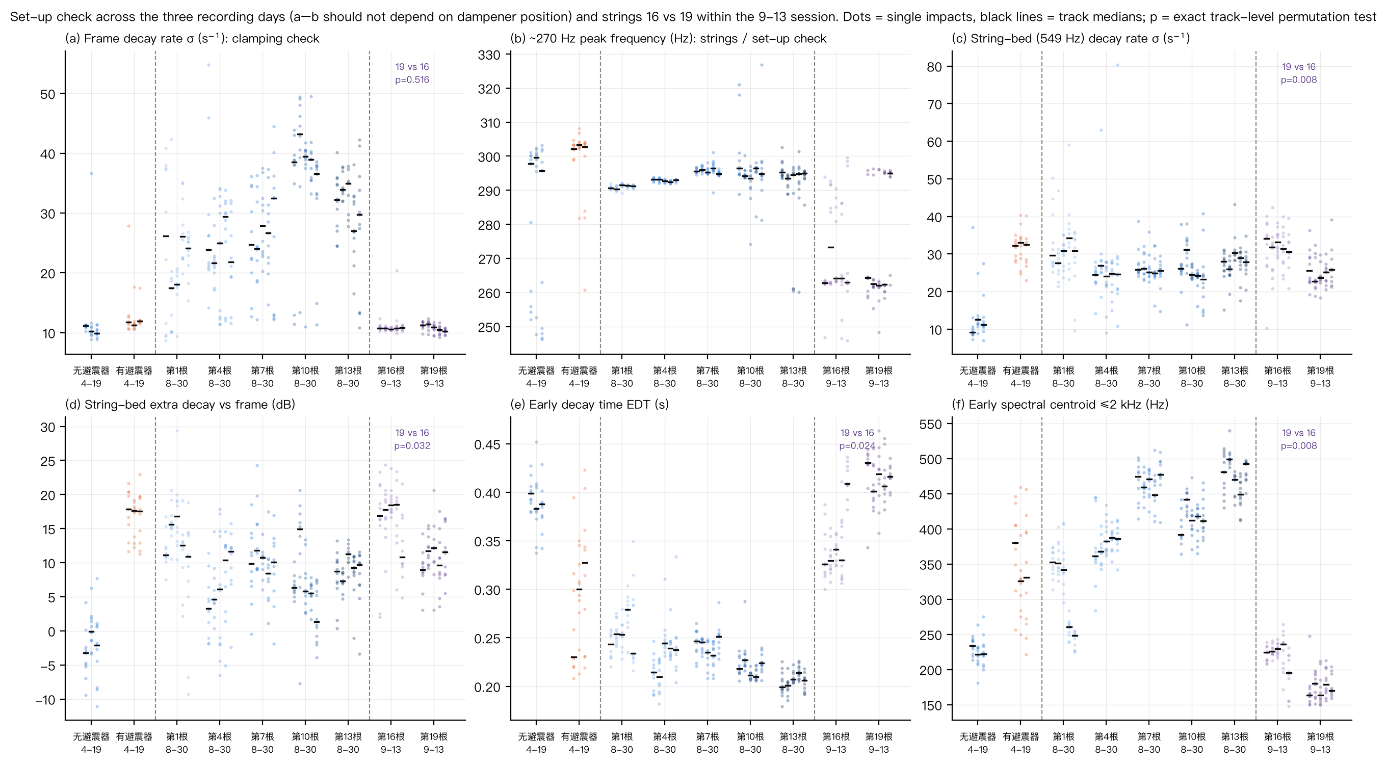
Figure 12. Setup consistency checks across the three recording sessions and position comparison within session B2. (a) Frame mode decay rate and (b) ~270 Hz mode peak frequency are in theory unrelated to dampener position, yet differ clearly between recording sessions; (c) the string-bed mode decay rate at all positions is comparable to the "with dampener" control; (d–f) comparison of cross strings 16 and 19, with the track-level exact permutation p in the upper right. Dots = single impacts, black lines = track medians.
5 Discussion
5.1 Main Findings Compared with Theory and the Literature
Using acoustic methods, this study reproduces the classic conclusion of mechanical measurements: the dampener strongly suppresses the string-bed mode and does not change the frame mode (Brody, 1989; Stroede et al., 1999; Li et al., 2004). Three independent lines of evidence support this: (i) the disappearance of the 549 Hz peak in the spectrum (Figure 5); (ii) narrowband envelopes showing the string-bed mode decay rate rising from 12.7 to 31.6 s⁻¹ and T60 shortening from 0.62 s to 0.22 s (Figure 6); (iii) the within-event relative quantity "extra decay of the string-bed mode relative to the frame mode" increasing by 18.9 dB (Figure 7). Leave-one-track-out cross-validation shows that the effect can be identified in every unseen recording and does not depend on any single recording.
Compared with the expectation in the experimental plan that "T60 shortens from about 1.1 s to 0.15 s (7-fold)," this study measured the string-bed mode T60 shortening from 0.62 s to 0.22 s (2.8-fold), and the loss factor increasing from 0.0074 to 0.0187 (2.5-fold); the direction agrees, but the factor is smaller than expected. Sources of the difference include that this experiment used ball-drop excitation with a clamped handle rather than plucking a string, and studied the whole string-bed mode rather than a single string.
The frame mode frequency (113–117 Hz) and decay rate are essentially the same under the two control conditions (11.3 vs 12.6 s⁻¹, T60 ≈ 0.6 s, η ≈ 0.03; identical fixed-window decay), showing that the first bending mode of the clamped racket is determined jointly by the clamp and the frame material, and that the dampener (≈ 0.7% of the frame mass) has no substantial effect on it (decay rate ratio 1.11, CI 0.89–1.35; mixed-effects model p = 0.04, an effect far smaller than for the string-bed mode). In the position groups, the frame mode frequency and decay rate drift together with recording order (Section 5.4), further showing that the frame mode is governed by clamping state rather than by the dampener. This agrees with the mechanical conclusion that "the dampener cannot reduce the low-frequency vibration transmitted to the arm"; therefore the value of the dampener lies mainly in sound and subjective feel, and it should not be expected to prevent tennis elbow.
5.2 Why Broadband T60 Is Insensitive but EDT Is Sensitive
Schroeder T60 is extrapolated from the −5…−25 dB segment of the EDC, but for impact-type signals the first 25 dB of energy decay is determined almost entirely by the 0–50 ms impact transient, and the fast-component decay rates under the two conditions are similar (≈ 30 s⁻¹). Without a dampener, the string-bed band (450–700 Hz) contributes only about 7% of the total energy and affects only the later part of the EDC. EDT and the residual energy fraction capture exactly this later part, so they are more suitable for evaluating "ringing." This methodological conclusion gives direct guidance for similar student experiments: do not report only a T60.
5.3 Two Mechanisms for the Mounting Position Effect
The B1 data support "the closer the dampener is to the center of the string bed, the less residual ringing after impact and the brighter the impact sound," and the B2 data further suggest that the effect weakens past the center; but judgments about both the shape and the mechanism require caution:
- Mode-shape damping mechanism (H5) predicts an effect proportional to sin²(πj/N), saturating at the center. This fits the saturating trends of the 435 Hz mode relative level and the low-frequency fraction, but not the monotonic decrease of the residual energy fraction and EDT (Table 3).
- Changed-excitation mechanism The ball lands at the center of the string bed, so moving the dampener toward the center means moving it toward the impact point. A rubber block near the contact region changes the local contact stiffness and effective mass, making the impact shorter and sharper; this is exactly what the rise of the early spectral centroid, high-frequency fraction, and impact peak with position indicates. The decrease in the ringing energy fraction may come mainly from an increase in the denominator (impact energy) rather than a decrease in the numerator. The fact that neither the broadband envelope decay rate nor the frame decay rate changes with position also supports "the change is in the excitation, not in the damping."
The two mechanisms are not mutually exclusive. Given that the 549 Hz string-bed mode has already been fully suppressed (at all seven positions the string-bed mode decay rate is comparable to the with-dampener control; 4.9), what the position experiments actually observe are secondary effects.
Cross strings 16 and 19 in B2 provide a new piece of information, but it does not distinguish between these two mechanisms: the ball lands near the center of the string bed, so both mode-shape damping (peak at cross string 10) and changed excitation (peak at the impact point) predict that "the effect weakens past the center," and cross string 19 being weaker than cross string 16 is compatible with both. What it really rules out is a third explanation: that the monotonic trend in B1 is merely setup drift along the recording order, or a monotonic "the closer to the head, the better" relationship. If that were the case, cross string 19, recorded in sequence in B2, should continue the B1 direction (less ringing), but in fact the opposite is seen. To distinguish mode-shape damping from changed excitation, it is still necessary to vary the ball impact point within the same session and to add a no-dampener baseline.
5.4 Limitations and Confounders
- Non-interleaved between-group comparison. The two conditions in dataset A consist of 3 recordings each, recorded consecutively; any setup change occurring between the two groups (clamping, microphone position, drop height) is confounded with the dampener. The 1.4% difference in frame mode frequency and the 1.9-fold difference in impact peak suggest that such differences did exist. Fortunately, the primary endpoints are within-event relative quantities (string-bed mode relative to frame mode) and are immune to gain and distance; and the invariance of the frame mode decay rate indicates that the clamping damping did not change systematically.
- Position fully confounded with recording order. The position groups were recorded in the order 1→13. During this time the noise floor dropped starting from track 4 of cross string 7 and returned to its original level in the first three tracks of cross string 13, and the frame mode frequency drifted by a net +2.3 Hz (not strictly monotonically). Although the main position metrics are gain-independent quantities, we cannot rule out that slow drifts in drop height or microphone position contributed part of the trend.
- No same-day baseline, no repeated mounting. The position groups lack a no-dampener baseline, and the dampener was mounted only once at each position, so mounting variation such as how deeply the dampener was pressed in cannot be assessed.
- Sample hierarchy. With 3 recordings per condition, the smallest p of the track-level test is 0.10; the very small p-values of the event-level mixed-effects models assume that impacts within a recording are exchangeable, and should be taken as measures of the direction and size of the effect rather than as strict hypothesis-test evidence.
- Indirectness of acoustic measurement. The microphone records radiated sound, and different modes have different radiation efficiencies; this paper does not compare absolute energies between modes, only the decay of the same mode under different conditions.
- Incomplete recording of experimental parameters. Drop height, microphone distance, and racket model/tension were not recorded track by track, which limits quantitative comparison with the literature.
- Different setup states on different recording sessions. The frame mode decay rate (about 11, 24–39, 11 s⁻¹) and the ~270 Hz mode peak frequency (about 300, 293, 263 Hz) differ clearly across the three recording sessions, although these quantities are unrelated to dampener position; there is also no common reference condition (the same position or a no-dampener baseline) that could "bridge" the recording sessions. Therefore B1 and B2 can only be compared within each session, and the cross-session pooled models are only exploratory. B2 has only two positions, also recorded in sequence, and there is a frame frequency drift of about 3 Hz within that session.
5.5 Recommendations for Future Experiments
- Use an ABAB interleaved design: without → with → without → with, ≥ 3 recordings each; in position experiments, record one no-dampener baseline before and after each position, and randomize the order of positions.
- Record the same set of reference conditions in every recording session (for example, no dampener + cross string 10), so that data from different sessions can be bridged onto the same scale; it is precisely the lack of this link between B1 and B2 in this study that prevented merging them.
- Cover the whole main string with positions (for example, cross strings 1, 4, 7, 10, 13, 16, 19) and complete them in random order within the same day, to test directly the falling part of the sin² curve past the center.
- Fix and record the drop height (guide tube), microphone distance (with a ruler), and frame clamping torque; record 5 s of silence before each recording for noise-floor calibration.
- Add a handle accelerometer (phone phyphox or MPU-6050) synchronized with the acoustics, to verify directly that "frame vibration is unchanged."
- In position experiments, also vary the ball impact point (center vs toward the throat vs toward the head), to distinguish the mode-shape damping and changed-excitation mechanisms.
- In the analysis, keep the mode-resolved metrics of this paper (string-bed mode extra decay, tail relative level) as primary endpoints.
6 Conclusions
- The string vibration dampener raises the decay rate of the string-bed fundamental mode (549 Hz) from 12.7 to 31.6 s⁻¹ (ratio 2.5, 95% CI 2.1–3.0; T60 shortens from 0.62 s to 0.22 s), and its extra decay relative to the frame mode increases by 18.9 dB (95% CI 16.3–21.4). The effect size is very large (g ≈ 3.5–4.9), and in leave-one-track-out cross-validation the presence or absence of the dampener is distinguished with 93–98% accuracy.
- The decay of the first frame bending mode (118 Hz) is essentially unaffected by the dampener (identical fixed-window decay; decay rate ratio 1.11, CI 0.89–1.35), confirming that the dampener does not change the low-frequency frame vibration transmitted to the arm. The 1.6 Hz difference in frame frequency between the two groups is in the direction opposite to mass loading and is attributed to different clamping states in the two groups of recordings (Section 5.4).
- In broadband terms, the dampener halves the residual energy fraction after 50 ms and shortens EDT by 25%; whereas the Schroeder T60 of the −5…−25 dB segment and the slow component of the broadband two-exponential model (dominated by the frame's long tail) hardly change. This shows that impact ringing should be evaluated with EDT and the residual energy fraction, and preferably with mode-resolved metrics.
- With the dampener mounted at any cross string from 1 to 19, the string-bed mode decay rate (24–32 s⁻¹) is far from the 11 s⁻¹ of the no-dampener control and close to the 32 s⁻¹ of the with-dampener control (cross-session comparison, qualitative); that is, mounting position does not determine "whether there is an effect," only the size of secondary effects.
- Within the same recording session, as the dampener moves from the throat to cross string 13, residual ringing decreases overall (54% lower at cross string 13 than at cross string 1, track-level ρ = −0.91) and the impact sound becomes brighter; over the range 1–13, the linear model outperforms the sin² mode-shape model. In the other recording session, cross string 19 shows slower string-bed mode decay, about 6 dB less extra decay, and a longer EDT than cross string 16; that is, the effect weakens past the center of the string bed. The exploratory pooled models favor sin² for some endpoints, but the same models can also be "fooled" into a sin² shape by recording drift. Because the setup state differed clearly between the two recording sessions and position is confounded with recording order within each session, the exact shape of the position effect, and whether it comes from mode-shape damping or from changed impact excitation, still need to be confirmed in an experiment performed on a single day, in random order, with reference conditions.
- Methodologically, this study establishes a complete, reproducible pipeline, from decoding Audacity projects, through event detection and quality control and noise-aware modal decay estimation, to hierarchical statistics and cross-validation, which is suitable as an analysis template for high-school acoustics experiments.
References
- Brody H. (1989). Vibration damping of tennis rackets. International Journal of Sport Biomechanics, 5(4), 451–456.
- Stroede C. L., Noble L., Walker H. S. (1999). The effect of tennis racket string vibration dampers on racket handle vibrations and discomfort following impacts. Journal of Sports Sciences, 17(5), 379–385.
- Li F.-X., Fewtrell D., Jenkins M. (2004). String vibration dampers do not reduce racket frame vibration transfer to the forearm. Journal of Sports Sciences, 22(11–12), 1041–1052.
- Brody H., Cross R., Lindsey C. (2002). The Physics and Technology of Tennis. Racquet Tech Publishing.
- Cross R. (1998). The sweet spots of a tennis racket. Sports Engineering, 1(2), 63–78.
- Schroeder M. R. (1965). New method of measuring reverberation time. Journal of the Acoustical Society of America, 37(3), 409–412.
- ISO 3382-1:2009. Acoustics — Measurement of room acoustic parameters — Part 1: Performance spaces.
- Ewins D. J. (2000). Modal Testing: Theory, Practice and Application (2nd ed.). Research Studies Press.
- Hedges L. V. (1981). Distribution theory for Glass's estimator of effect size and related estimators. Journal of Educational Statistics, 6(2), 107–128.
- Seabold S., Perktold J. (2010). statsmodels: Econometric and statistical modeling with Python. Proceedings of the 9th Python in Science Conference, 92–96.
Open the recording files
The student recorded in Audacity, which saves .aup3 files. It looks like an audio file but is really a small : the sound is cut into “blocks” of a few hundred thousand numbers each. A short program stitches the blocks back in the order the project records, giving one long list of numbers per recording.
There are 44,100 numbers per second (a of 44.1 kHz); each is how far the mic's membrane was pushed at that instant.
Check the raw sound first
Three things: any (sound so loud it's flattened — none); are the numbers truly high-precision (yes); and how noisy is the quiet part — the . The noise floor comes back again and again: it's the yardstick for “this is a real sound”.
Find every ball drop
The rule is simple: a spike at least 100× louder than the noise floor, and spikes at least 1.5 s apart (a drop rings for under a second, so one drop is never counted twice). From each spike, step backward to the first point where the previous 2 ms were quiet — that's where the drop starts. Drag the threshold yourself:
The vertical axis is a log scale: each step up is 10× louder, so tiny noise and huge hits fit on one chart.
Clean: which drops can't be used
The ball bounces up and lands again (a ), and the second hit covers the first one's ringing. So each drop's analysis window is cut just before any rebound. Then drops are removed by rules written in advance:
| Rule | Why | # |
|---|---|---|
| Rebound within 0.25 s | too little clean ringing left | 8 |
| Window under 0.3 s after cutting | same reason | 7 |
| Hit less than half the recording's usual strength | ball missed the centre | 5 |
| Too close to the end of a recording | ringing cut off | 1 |
Removed drops aren't deleted — just flagged — so anyone can check why each one was dropped.
Measure: turn each drop into a few numbers
For each good drop:
- Filter: a keeps one mode, e.g. the 530–570 Hz ping — like listening to one voice in a crowd.
- Envelope: average the loudness every 2.5 ms to get a smooth loudness-over-time curve, in decibels.
- Fit: on the decibel chart, from 10 ms after the peak until the curve nears the noise floor (noise + 10 dB), draw the best straight line. Its slope is σ.
- Compare: also compute “how many more decibels the string-bed mode faded than the frame mode”. Because it compares a drop with itself, recording volume and mic distance can't affect it.
A real example: drop #4 in the first “no dampener” recording — ping σ = 9.7 s⁻¹ (T60 0.71 s), frame σ = 11.3 s⁻¹.
Compare fairly
An easy mistake: the control set has 62 drops, but they come from 6 recordings. The 10 drops in one recording share the clamp, the mic and the room — they're alike, not 10 separate pieces of evidence. So we first take each recording's , then compare recording to recording.
How do we know a difference isn't luck? With a : if position truly had no effect, the “which recording belongs to which position” labels would be arbitrary. Shuffle the labels and see whether random labelling produces a gap this big. Try it (data: ping decay rates of the 5 recordings each at strings 16 and 19, on 09-13):
Two more tools: the says how big a difference is; the says how precise it is. The only answers “could it be luck?” — you need all three.
Test on data the method hasn't seen
That's the “hide a recording and guess” exam from Part 1, section 6. A pattern that only works on recordings it has already seen is just a memorised answer. Ours held on every hidden recording.
Check, and check again
- Check against someone else's answer: the student had exported some audio from Audacity. Our program's numbers matched Audacity's export exactly, so step 1 read the files correctly.
- Look with your own eyes: every detected start in all 41 recordings was drawn and checked one by one — no missed drops, no rebound counted as a new drop.
- Start over from scratch: delete all intermediate results, rebuild from the raw files to the final charts with one command — identical results.
- Never ignore an “impossible” number: once, the noise came out louder than the signal — impossible. Tracing it showed a side effect of the filter: it smears the hit about 0.1 s backward in time, polluting the stretch used to measure noise. After the fix, one earlier conclusion had to be withdrawn.
To be honest: some rules were adjusted after seeing part of the results. The biggest one: 549 Hz became the main measure partly because we saw it change with the dampener. So the strongest test is to run today's fixed rules, unchanged, on a brand-new batch of recordings.
Tools we used
Free recording and editing software. All the sound was recorded with it.
A programming language. The whole analysis is a dozen or so small Python programs.
A small database. An .aup3 file is one of these, so this is how the sound gets read out.
For working with long lists of numbers, e.g. averaging 1.8 million samples at once.
A science toolbox: filters, spike-finding and curve-fitting all come from here.
For tables — Excel you can program: one row per drop, one column per measure.
For charts. Every figure in the paper was drawn with it.
Statistics and machine learning: the recording-level tests and the cross-validation exam.
A notebook where you write code and see results side by side. Your six practice lessons use it.
Glossary
Words with a dotted underline in the text can also be tapped for an explanation.